STEP 1: Pure Random Walk - The Foundation

Mathematical Formulation

Discrete Time Random Walk: \[X_n = X_{n-1} + \epsilon_n\]

Where:

- \(X_n\) = position at step \(n\)

- \(X_0 = 0\) (starting position)

- \(\epsilon_n \sim \mathcal{N}(0, \sigma^2)\) (random increment)

Direct Simulation Code

# ==============================================================================
# STEP 1: PURE RANDOM WALK - NO DRIFT, NO BOUNDARIES
# ==============================================================================

# PARAMETERS
n_steps <- 500        # Number of steps to simulate
sigma <- 3            # Standard deviation of noise

# SIMULATION
# set.seed(123)
X <- numeric(n_steps + 1)  # Pre-allocate vector
X[1] <- 0                   # Starting position

# Generate the random walk step by step
for (n in 2:(n_steps + 1)) {
  epsilon <- rnorm(1, mean = 0, sd = sigma)  # Random increment
  X[n] <- X[n-1] + epsilon                    # Update position
}

# VISUALIZATION
steps <- 0:n_steps
plot(steps, X, type = "l", col = "steelblue", lwd = 2,
     main = "Step 1: Pure Random Walk",
     xlab = "Step (n)", ylab = "Position X(n)")
abline(h = 0, lty = 2, col = "gray")
grid()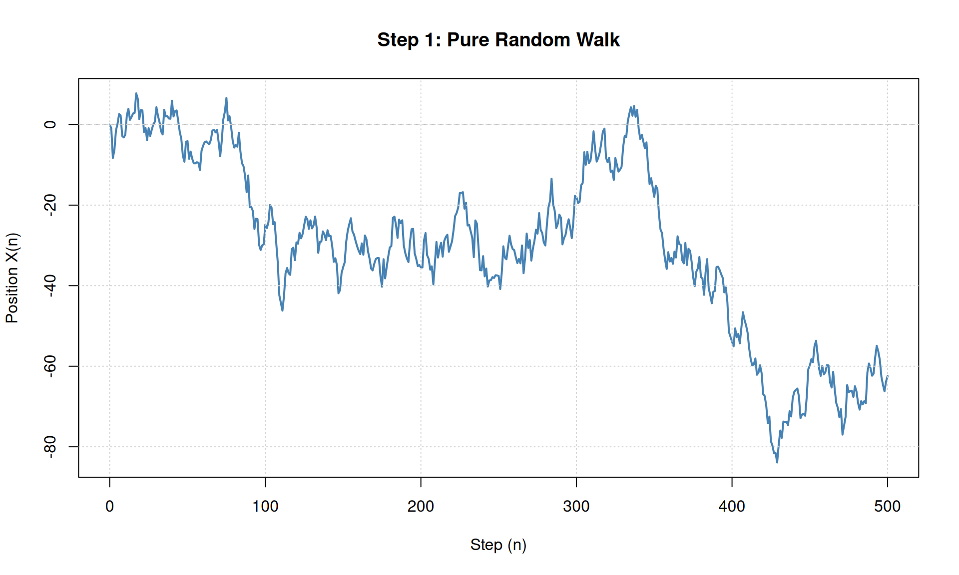

# KEY OBSERVATION: The walk has no direction - just random noise
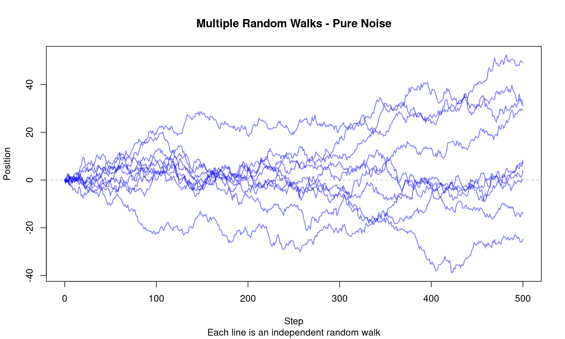
cat("Final position:", X[n_steps + 1], "\n")

## Final position: -62.44304

Multiple Paths to See Variability

# Simulate multiple random walks to see the pattern
n_paths <- 10
n_steps <- 500

# Store all paths in a matrix
all_paths <- matrix(0, nrow = n_steps + 1, ncol = n_paths)

set.seed(456)
for (path_id in 1:n_paths) {
  X <- numeric(n_steps + 1)
  X[1] <- 0
  
  for (n in 2:(n_steps + 1)) {
    epsilon <- rnorm(1, mean = 0, sd = 1)
    X[n] <- X[n-1] + epsilon
  }
  
  all_paths[, path_id] <- X
}

# Plot all paths
plot(0:n_steps, all_paths[, 1], type = "n", 
     ylim = range(all_paths),
     main = "Multiple Random Walks - Pure Noise",
     xlab = "Step", ylab = "Position",
     sub = "Each line is an independent random walk")
abline(h = 0, lty = 2, col = "gray")

for (i in 1:n_paths) {
  lines(0:n_steps, all_paths[, i], col = rgb(0, 0, 1, 0.5), lwd = 1.5)
}

STEP 2: Adding Drift - Systematic Tendency

Mathematical Formulation

Random Walk with Drift: \[X_n = X_{n-1} + \mu + \epsilon_n\]

Where:

- \(\mu\) = drift parameter (systematic tendency per step)

- Positive \(\mu\) → upward tendency

- Negative \(\mu\) → downward tendency

Direct Simulation with Drift

# ==============================================================================
# STEP 2: RANDOM WALK WITH DRIFT
# ==============================================================================

# PARAMETERS
n_steps <- 500
mu <- -0.1             # Drift parameter
sigma <- 1            # Noise standard deviation

# SIMULATION
# set.seed(789)
X <- numeric(n_steps + 1)
X[1] <- 0

for (n in 2:(n_steps + 1)) {
  epsilon <- rnorm(1, mean = 0, sd = sigma)
  X[n] <- X[n-1] + mu + epsilon  # Now includes drift
}

# VISUALIZATION
plot(0:n_steps, X, type = "l", col = "darkgreen", lwd = 2,
     main = paste("Step 2: Random Walk with Drift (μ =", mu, ")"),
     xlab = "Step", ylab = "Position")
abline(h = 0, lty = 2, col = "gray")
abline(0, mu, col = "red", lwd = 2, lty = 2)  # Expected trajectory
legend("topleft", 
       legend = c("Actual path", "Expected path (μ × n)"),
       col = c("darkgreen", "red"), lwd = 2, lty = c(1, 2))
grid()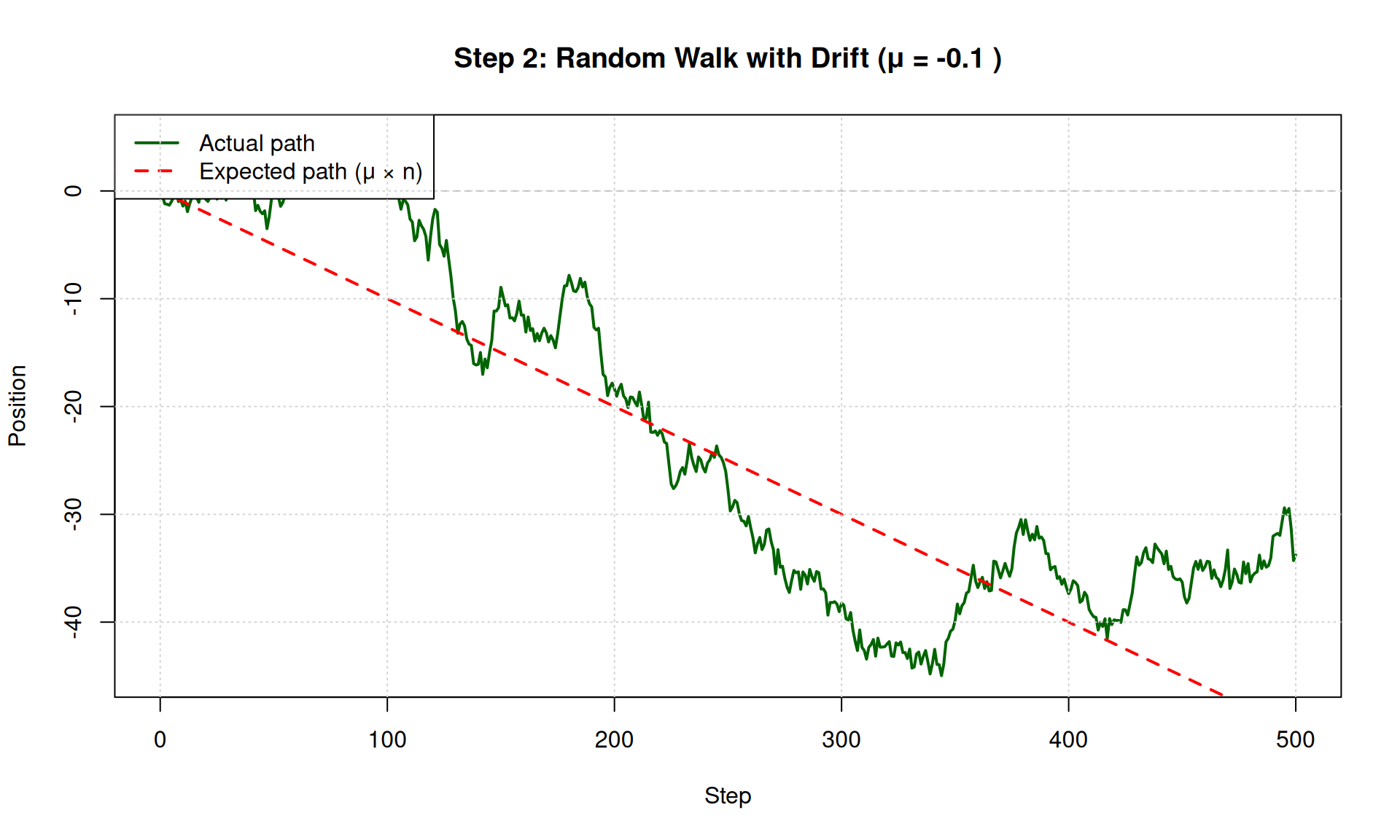

cat("Starting position:", X[1], "\n")

## Starting position: 0

cat("Final position:", X[n_steps + 1], "\n")

## Final position: -33.7729

cat("Expected final position (μ × n):", mu * n_steps, "\n")

## Expected final position (μ × n): -50

Compare Different Drift Values

# Compare mu = -0.2, 0, +0.2
drift_values <- c(-0.2, 0, 0.2)
n_steps <- 500
colors <- c("red", "gray", "blue")

# Setup plot
plot(0:n_steps, 0:n_steps, type = "n", 
     ylim = c(-150, 150),
     main = "Effect of Drift Parameter",
     xlab = "Step", ylab = "Position")
abline(h = 0, lty = 2)
grid()

set.seed(100)
for (i in 1:3) {
  mu <- drift_values[i]
  
  X <- numeric(n_steps + 1)
  X[1] <- 0
  
  for (n in 2:(n_steps + 1)) {
    epsilon <- rnorm(1, mean = 0, sd = 1)
    X[n] <- X[n-1] + mu + epsilon
  }
  
  lines(0:n_steps, X, col = colors[i], lwd = 2)
}

legend("topleft", 
       legend = paste("μ =", drift_values),
       col = colors, lwd = 2)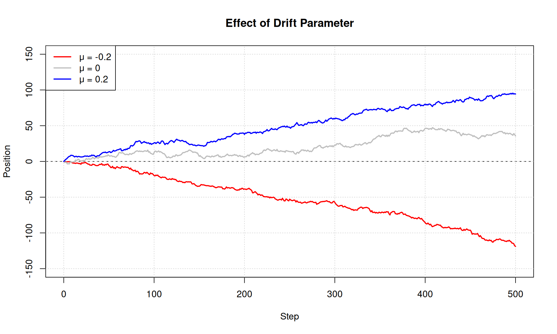

STEP 3: From Discrete to Continuous Time

Mathematical Formulation

Continuous Time Approximation: \[X(t + \Delta t) = X(t) + v \cdot \Delta t + s \cdot \sqrt{\Delta t} \cdot Z\]

Where:

- \(t\) = continuous time (in seconds)

- \(\Delta t\) = time step size (e.g., 0.001 seconds)

- \(v\) = drift rate (evidence per second)

- \(s\) = diffusion coefficient (noise intensity) - \(Z \sim \mathcal{N}(0, 1)\)

KEY: Why \(\sqrt{\Delta t}\)?

- Preserves correct variance scaling in continuous limit

- Ensures Var[noise] = \(s^2 \cdot \Delta t\) per time step

Direct Simulation in Continuous Time

# ==============================================================================
# STEP 3: CONTINUOUS TIME APPROXIMATION (EULER-MARUYAMA)
# ==============================================================================

# PARAMETERS
v <- 0.3              # Drift rate (evidence per second)
s <- 1.0              # Diffusion coefficient (noise intensity)
dt <- 0.001           # Time step (1 millisecond)
T_max <- 2.0          # Maximum time (seconds)

# SIMULATION
n_steps <- round(T_max / dt)
time <- seq(0, T_max, by = dt)
X <- numeric(n_steps + 1)
X[1] <- 0

for (i in 2:(n_steps + 1)) {
  Z <- rnorm(1, mean = 0, sd = 1)
  X[i] <- X[i-1] + v * dt + s * sqrt(dt) * Z
}

# VISUALIZATION
plot(time, X, type = "l", col = "purple", lwd = 2,
     main = "Step 3: Continuous Time Random Walk (Wiener Process)",
     xlab = "Time (seconds)", ylab = "Evidence X(t)",
     sub = paste("v =", v, ", s =", s, ", Δt =", dt))
abline(h = 0, lty = 2, col = "gray")
abline(0, v, col = "red", lwd = 2, lty = 2)
grid()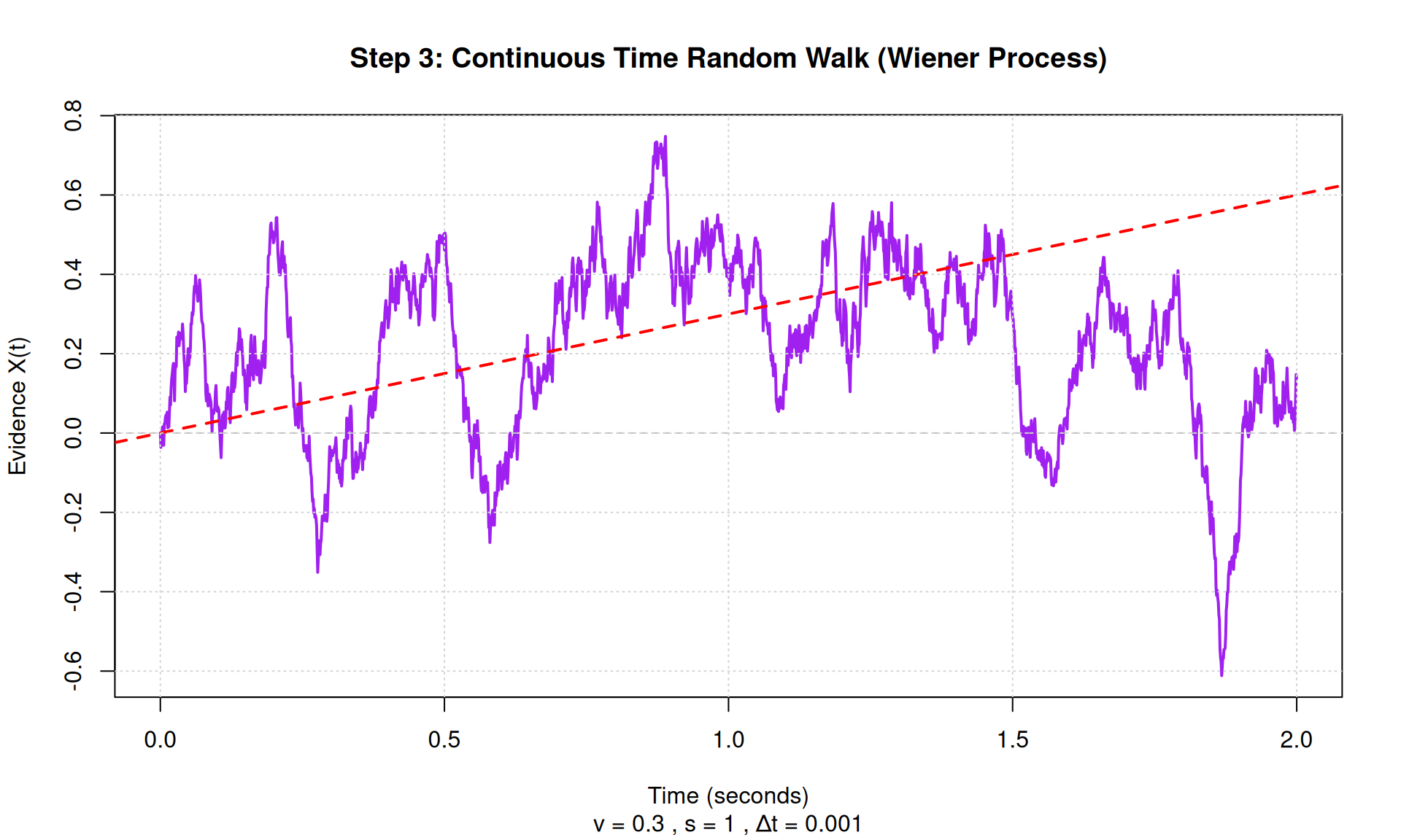

cat("Total time simulated:", T_max, "seconds\n")

## Total time simulated: 2 seconds

cat("Number of time steps:", n_steps, "\n")

## Number of time steps: 2000

cat("Final position:", round(X[length(X)], 2), "\n")

## Final position: 0.14

STEP 4: Adding Decision Boundaries

Mathematical Formulation

Decision Rule:

- Upper boundary at \(X = a\) → Decision “A” (e.g., “yes”, “correct”)

- Lower boundary at \(X = 0\) → Decision “B” (e.g., “no”, “error”)

- Starting point at \(X = z\) (typically \(z = a/2\) for unbiased)

Process:

1. Start at \(X(0) = z\)

2. Accumulate evidence: \(X(t + \Delta t) = X(t) + v \cdot \Delta t + s \cdot \sqrt{\Delta t} \cdot Z\)

3. Stop when \(X(t) \geq a\) OR \(X(t) \leq 0\)

4. Record: choice (which boundary) and RT (time to boundary)

Direct Simulation with Boundaries

# ==============================================================================
# STEP 4A: SEE THE RANDOM WALKS WITH BOUNDARIES
# ==============================================================================

# PARAMETERS
v <- 0.1             # Drift rate (moderate)
a <- 2.0              # Boundary separation
z <- 0.5 * a          # Starting point (middle)
s <- 1.0              # Diffusion coefficient
dt <- 0.001           # Time step
max_time <- 2.0       # Maximum time
n_paths <- 15         # Number of paths to show

# Storage for all paths
all_paths <- list()
all_times <- list()
all_choices <- character(n_paths)
all_RTs <- numeric(n_paths)

set.seed(222)
cat("Simulating", n_paths, "visible paths...\n\n")

## Simulating 15 visible paths...

# Simulate each path
for (path_id in 1:n_paths) {
  evidence <- z
  time_elapsed <- 0
  step_counter <- 0

  # Store this path
  evidence_path <- evidence
  time_path <- 0

  # Run until boundary hit
  while (evidence > 0 && evidence < a && time_elapsed < max_time) {
    Z <- rnorm(1, 0, 1)
    evidence <- evidence + v * dt + s * sqrt(dt) * Z
    time_elapsed <- time_elapsed + dt
    step_counter <- step_counter + 1

    # Store every 10th point to keep file size manageable
    if (step_counter %% 10 == 0) {
      evidence_path <- c(evidence_path, evidence)
      time_path <- c(time_path, time_elapsed)
    }
  }

  # Always store the final point where boundary was hit
  evidence_path <- c(evidence_path, evidence)
  time_path <- c(time_path, time_elapsed)

  # Record outcome
  if (time_elapsed >= max_time) {
    all_choices[path_id] <- "Timeout"
    all_RTs[path_id] <- NA
  } else {
    all_choices[path_id] <- ifelse(evidence >= a, "Upper", "Lower")
    all_RTs[path_id] <- time_elapsed
  }

  # Store path
  all_paths[[path_id]] <- evidence_path
  all_times[[path_id]] <- time_path
  
  cat("Path", path_id, ":", all_choices[path_id], "boundary, RT =", 
      round(all_RTs[path_id], 3), "s\n")
}

## Path 1 : Timeout boundary, RT = NA s
## Path 2 : Lower boundary, RT = 0.365 s
## Path 3 : Lower boundary, RT = 0.097 s
## Path 4 : Lower boundary, RT = 0.92 s
## Path 5 : Upper boundary, RT = 0.359 s
## Path 6 : Lower boundary, RT = 1.03 s
## Path 7 : Lower boundary, RT = 1.82 s
## Path 8 : Lower boundary, RT = 0.363 s
## Path 9 : Lower boundary, RT = 1.044 s
## Path 10 : Upper boundary, RT = 0.471 s
## Path 11 : Upper boundary, RT = 0.384 s
## Path 12 : Lower boundary, RT = 0.856 s
## Path 13 : Upper boundary, RT = 0.432 s
## Path 14 : Upper boundary, RT = 0.628 s
## Path 15 : Upper boundary, RT = 0.536 s

# VISUALIZATION: All paths on one plot
plot(NULL, xlim = c(0, max_time), ylim = c(-0.15, a + 0.15),
     main = "Step 4: Evidence Paths with Decision Boundaries",
     xlab = "Time (seconds)", ylab = "Evidence",
     sub = paste(n_paths, "independent random walks"))

# Draw boundaries FIRST (so paths go on top)
abline(h = a, col = "red", lwd = 3, lty = 1)
abline(h = 0, col = "red", lwd = 3, lty = 1)
abline(h = z, col = "orange", lwd = 2, lty = 2)

# Add labels
text(max_time * 0.98, a + 0.08, "UPPER BOUNDARY", col = "red", adj = 1, font = 2)
text(max_time * 0.98, -0.08, "LOWER BOUNDARY", col = "red", adj = 1, font = 2)
text(0.05, z + 0.08, "START", col = "orange", adj = 0)

# Draw each path
for (i in 1:n_paths) {
  # Color based on which boundary was hit
  if (all_choices[i] == "Upper") {
    path_color <- rgb(0, 0, 0.8, 0.6)  # Blue for upper
  } else if (all_choices[i] == "Lower") {
    path_color <- rgb(0.8, 0, 0, 0.6)  # Red for lower  
  } else {
    path_color <- rgb(0.5, 0.5, 0.5, 0.4)  # Gray for timeout
  }
  
  lines(all_times[[i]], all_paths[[i]], col = path_color, lwd = 1.5)
}

# Add legend
legend("topleft", 
       legend = c("Upper boundary", "Lower boundary", "Timeout"),
       col = c(rgb(0, 0, 0.8, 0.6), rgb(0.8, 0, 0, 0.6), rgb(0.5, 0.5, 0.5, 0.4)),
       lwd = 2, bg = "white")

grid()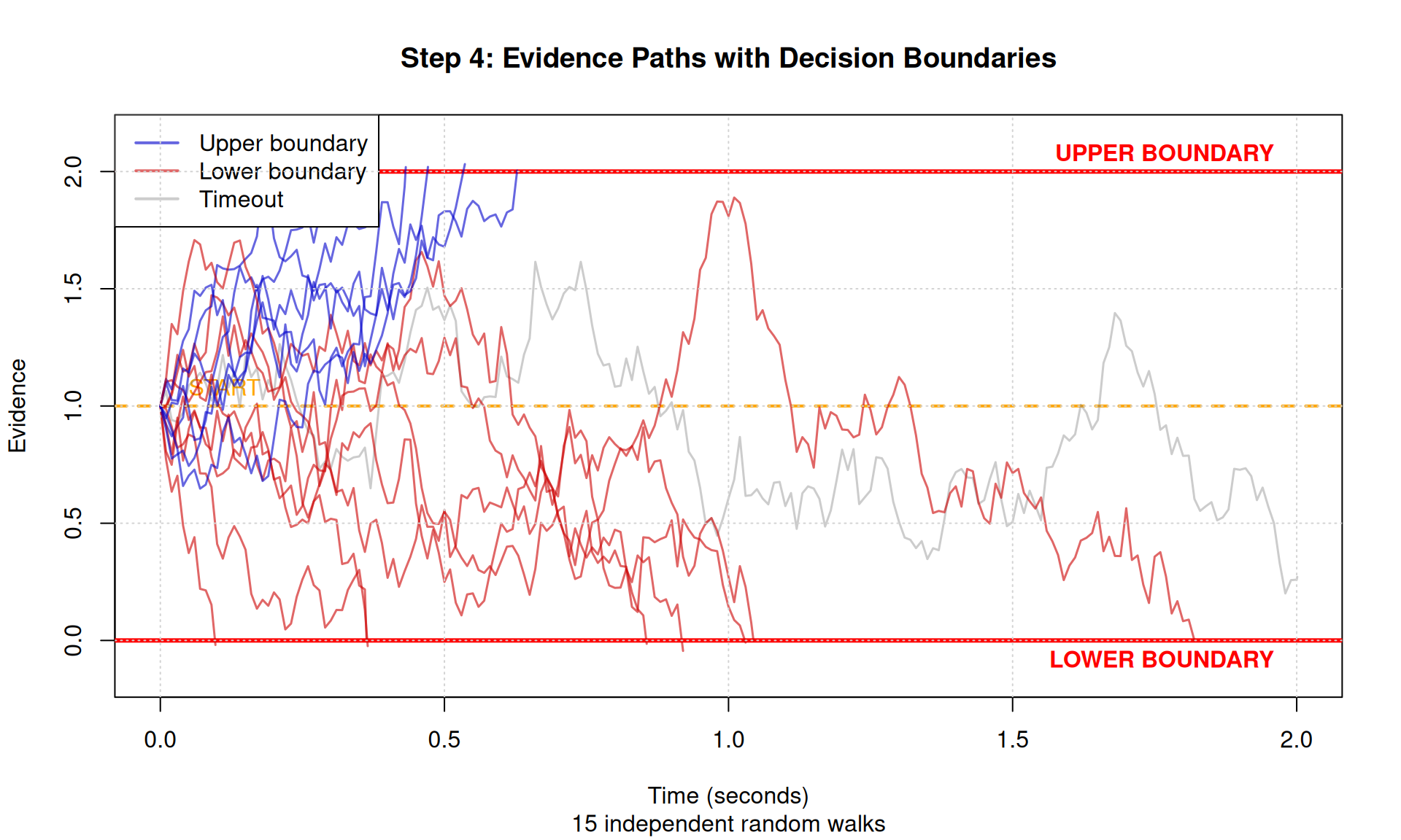

# Summary
cat("\n=== SUMMARY ===\n")

## 
## === SUMMARY ===

cat("Upper boundary:", sum(all_choices == "Upper"), "/", n_paths, "\n")

## Upper boundary: 6 / 15

cat("Lower boundary:", sum(all_choices == "Lower"), "/", n_paths, "\n")

## Lower boundary: 8 / 15

cat("Timeouts:", sum(all_choices == "Timeout"), "/", n_paths, "\n")

## Timeouts: 1 / 15

Key Observations

Look at the plot above and notice:

All paths start at the same point (orange line)
Paths wander randomly but with upward drift (v > 0)
Blue paths hit upper boundary → these are “correct” responses
Red paths hit lower boundary → these are “errors”
Different RTs even for same boundary (randomness!)
More blue than red because drift favors upper boundary

Simulate Multiple Trials

# Simulate many trials to see distributions
n_trials <- 500
v <- 0.3
a <- 1.0
z <- 0.5 * a
s <- 1.0
dt <- 0.001
max_time <- 5.0

# Store results
choices <- character(n_trials)
RTs <- numeric(n_trials)

set.seed(333)
cat("Simulating", n_trials, "trials...\n")

## Simulating 500 trials...

for (trial in 1:n_trials) {
  evidence <- z
  time_elapsed <- 0
  
  while (evidence > 0 && evidence < a && time_elapsed < max_time) {
    Z <- rnorm(1, 0, 1)
    evidence <- evidence + v * dt + s * sqrt(dt) * Z
    time_elapsed <- time_elapsed + dt
  }
  
  if (time_elapsed >= max_time) {
    choices[trial] <- NA
    RTs[trial] <- NA
  } else {
    choices[trial] <- ifelse(evidence >= a, "Upper", "Lower")
    RTs[trial] <- time_elapsed
  }
}

# Remove NA trials
valid <- !is.na(choices)
choices <- choices[valid]
RTs <- RTs[valid]

# RESULTS
cat("\nResults from", sum(valid), "valid trials:\n")

## 
## Results from 500 valid trials:

cat("P(Upper boundary):", round(mean(choices == "Upper"), 3), "\n")

## P(Upper boundary): 0.582

cat("Mean RT:", round(mean(RTs), 3), "seconds\n")

## Mean RT: 0.264 seconds

cat("Mean RT (Upper):", round(mean(RTs[choices == "Upper"]), 3), "seconds\n")

## Mean RT (Upper): 0.274 seconds

cat("Mean RT (Lower):", round(mean(RTs[choices == "Lower"]), 3), "seconds\n")

## Mean RT (Lower): 0.251 seconds

# VISUALIZATION: RT Distributions
par(mfrow = c(1, 2))

# Histogram by choice
hist(RTs[choices == "Upper"], breaks = 30, col = rgb(0, 0, 1, 0.5),
     main = "RT Distributions by Choice",
     xlab = "Reaction Time (seconds)", xlim = range(RTs))
hist(RTs[choices == "Lower"], breaks = 30, col = rgb(1, 0, 0, 0.5), add = TRUE)
legend("topright", legend = c("Upper", "Lower"), 
       fill = c(rgb(0, 0, 1, 0.5), rgb(1, 0, 0, 0.5)))

# Overall RT distribution
hist(RTs, breaks = 30, col = "lightgray",
     main = "Overall RT Distribution",
     xlab = "Reaction Time (seconds)")
abline(v = mean(RTs), col = "red", lwd = 2)
text(mean(RTs), par("usr")[4] * 0.9, 
     paste("Mean =", round(mean(RTs), 3)), 
     col = "red", adj = 0)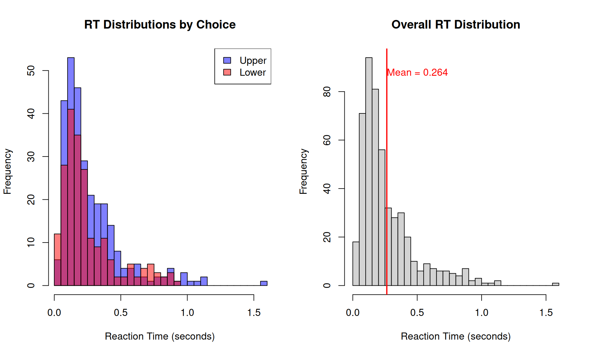

par(mfrow = c(1, 1))

STEP 5: Adding Non-Decision Time

Mathematical Formulation

Total RT = Decision Time + Non-Decision Time

\[RT_{total} = RT_{decision} + T_{er}\]

Where:

- \(RT_{decision}\) = time to reach boundary

- \(T_{er}\) = non-decision time (encoding + motor response)

- Typically \(T_{er}\) = 0.2 - 0.4 seconds

Simulation with Non-Decision Time

# ==============================================================================
# STEP 5: ADDING NON-DECISION TIME
# ==============================================================================

# PARAMETERS
v <- 0.3
a <- 1.0
z <- 0.5 * a
s <- 1.0
Ter <- 0.3            # Non-decision time (NEW!)
dt <- 0.001
max_time <- 5.0

# Simulate one trial
evidence <- z
decision_time <- 0

while (evidence > 0 && evidence < a && decision_time < max_time) {
  Z <- rnorm(1, 0, 1)
  evidence <- evidence + v * dt + s * sqrt(dt) * Z
  decision_time <- decision_time + dt
}

if (decision_time >= max_time) {
  choice <- NA
  RT_total <- NA
} else {
  choice <- ifelse(evidence >= a, "Upper", "Lower")
  RT_total <- decision_time + Ter  # Add non-decision time!
}

cat("Decision time:", round(decision_time, 3), "seconds\n")

## Decision time: 0.232 seconds

cat("Non-decision time:", Ter, "seconds\n")

## Non-decision time: 0.3 seconds

cat("Total RT:", round(RT_total, 3), "seconds\n")

## Total RT: 0.532 seconds

cat("Choice:", choice, "\n")

## Choice: Upper

# VISUALIZATION: Components of RT
barplot(c(decision_time, Ter), 
        names.arg = c("Decision Time", "Non-Decision Time"),
        col = c("steelblue", "orange"),
        main = "Components of Reaction Time",
        ylab = "Time (seconds)",
        ylim = c(0, RT_total * 1.2))
text(0.7, decision_time/2, round(decision_time, 3), col = "white")
text(1.9, decision_time + Ter/2, Ter, col = "white")
text(1.3, RT_total + 0.05, paste("Total RT =", round(RT_total, 3)))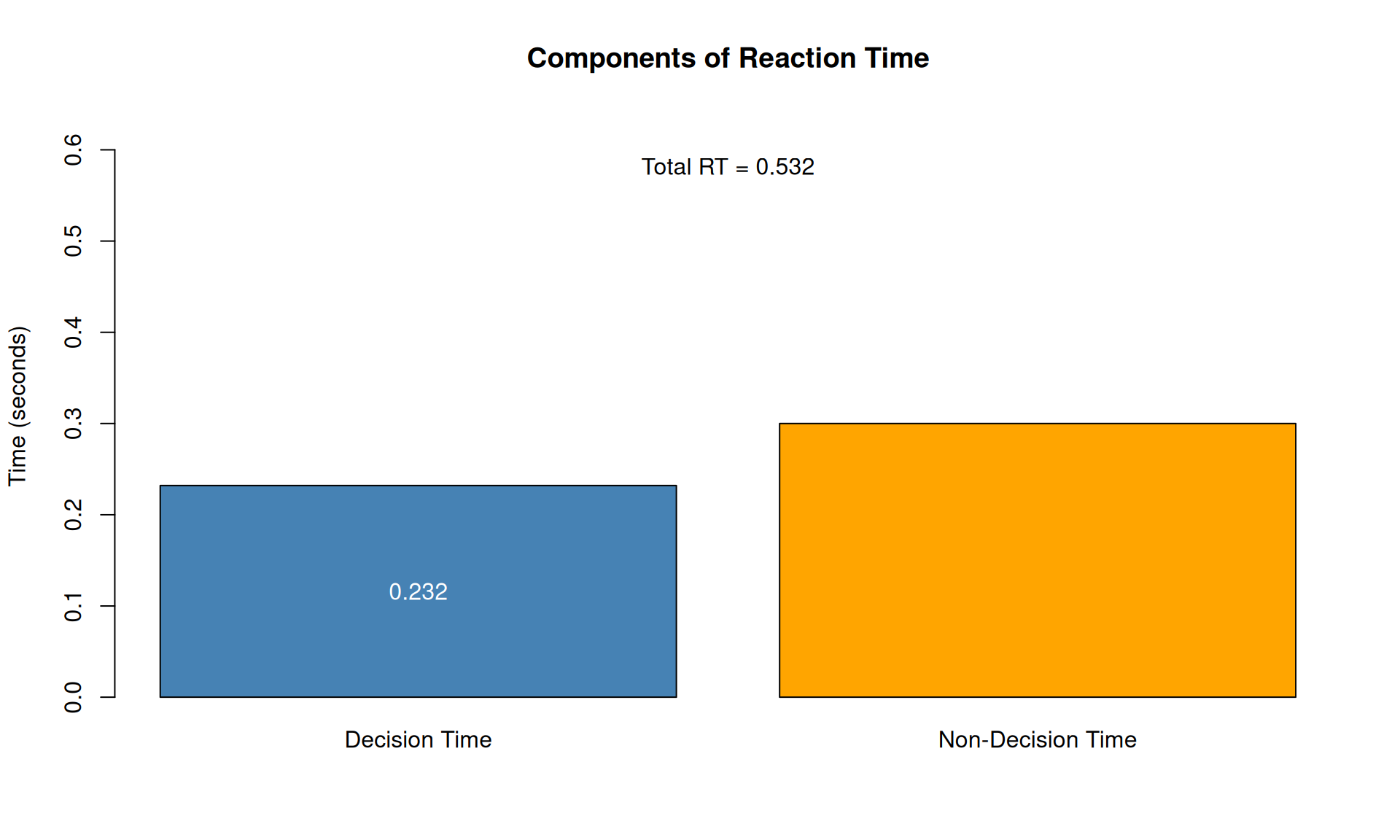

STEP 6: The Complete DDM

Mathematical Formulation

Full DDM Process:

Initialize: \(X(0) = z\)
Accumulate: \(X(t + \Delta t) = X(t) + v \cdot \Delta t + s \cdot \sqrt{\Delta t} \cdot Z\)
Decide: Stop when \(X(t) \geq a\) or \(X(t) \leq 0\)
Respond: \(RT = t_{decision} + T_{er}\)

Parameters:

- \(v\) = drift rate (quality of evidence)

\(a\) = boundary separation (speed-accuracy tradeoff)

- \(z\) = starting point (bias)

- \(s\) = diffusion coefficient (noise)

- \(T_{er}\) = non-decision time

Complete DDM Simulation

# ==============================================================================
# STEP 6: COMPLETE DDM - ALL PARAMETERS
# ==============================================================================

# PARAMETERS (All Together!)
v <- 0.25             # Drift rate
a <- 1.2              # Boundary separation
z_prop <- 0.5         # Starting point (as proportion)
z <- z_prop * a       # Convert to absolute
s <- 1.0              # Diffusion coefficient
Ter <- 0.25           # Non-decision time
dt <- 0.001           # Time step
max_time <- 10.0      # Max time

# Simulate many trials
n_trials <- 1000
all_choices <- character(n_trials)
all_RTs <- numeric(n_trials)

set.seed(555)
cat("Running complete DDM with", n_trials, "trials...\n\n")

## Running complete DDM with 1000 trials...

for (trial in 1:n_trials) {
  evidence <- z
  time <- 0
  
  while (evidence > 0 && evidence < a && time < max_time) {
    Z <- rnorm(1, 0, 1)
    evidence <- evidence + v * dt + s * sqrt(dt) * Z
    time <- time + dt
  }
  
  if (time >= max_time) {
    all_choices[trial] <- NA
    all_RTs[trial] <- NA
  } else {
    all_choices[trial] <- ifelse(evidence >= a, "Upper", "Lower")
    all_RTs[trial] <- time + Ter
  }
}

# Clean data
valid <- !is.na(all_choices)
choices <- all_choices[valid]
RTs <- all_RTs[valid]

# SUMMARY STATISTICS
cat("RESULTS:\n")

## RESULTS:

cat("Valid trials:", sum(valid), "/", n_trials, "\n")

## Valid trials: 1000 / 1000

cat("Accuracy (P(Upper)):", round(mean(choices == "Upper"), 3), "\n")

## Accuracy (P(Upper)): 0.607

cat("Mean RT:", round(mean(RTs), 3), "seconds\n")

## Mean RT: 0.631 seconds

cat("Median RT:", round(median(RTs), 3), "seconds\n")

## Median RT: 0.543 seconds

cat("SD RT:", round(sd(RTs), 3), "seconds\n\n")

## SD RT: 0.307 seconds

cat("By Choice:\n")

## By Choice:

cat("Upper - N:", sum(choices == "Upper"), 
    ", Mean RT:", round(mean(RTs[choices == "Upper"]), 3), "\n")

## Upper - N: 607 , Mean RT: 0.622

cat("Lower - N:", sum(choices == "Lower"), 
    ", Mean RT:", round(mean(RTs[choices == "Lower"]), 3), "\n")

## Lower - N: 393 , Mean RT: 0.643

# COMPREHENSIVE VISUALIZATION
par(mfrow = c(2, 2))

# 1. RT distributions by choice
hist(RTs[choices == "Upper"], breaks = 40, col = rgb(0, 0, 1, 0.5),
     main = "RT Distributions",
     xlab = "RT (seconds)", xlim = range(RTs), freq = FALSE)
hist(RTs[choices == "Lower"], breaks = 40, col = rgb(1, 0, 0, 0.5), 
     add = TRUE, freq = FALSE)
legend("topright", c("Upper", "Lower"), 
       fill = c(rgb(0, 0, 1, 0.5), rgb(1, 0, 0, 0.5)))

# 2. Choice proportions
choice_counts <- table(choices)
barplot(choice_counts, col = c("salmon", "steelblue"),
        main = "Choice Frequencies",
        ylab = "Count")

# 3. RT quantiles by choice
quantiles <- c(0.1, 0.3, 0.5, 0.7, 0.9)
q_upper <- quantile(RTs[choices == "Upper"], quantiles)
q_lower <- quantile(RTs[choices == "Lower"], quantiles)

plot(quantiles, q_upper, type = "b", col = "blue", lwd = 2,
     ylim = range(c(q_upper, q_lower)),
     main = "RT Quantiles by Choice",
     xlab = "Quantile", ylab = "RT (seconds)")
lines(quantiles, q_lower, type = "b", col = "red", lwd = 2)
legend("topleft", c("Upper", "Lower"), col = c("blue", "red"), lwd = 2)

# 4. Parameter summary
plot.new()
text(0.5, 0.8, "DDM Parameters", cex = 1.5, font = 2)
text(0.2, 0.6, "Drift rate (v):", adj = 0)
text(0.7, 0.6, v, adj = 0)
text(0.2, 0.5, "Boundary (a):", adj = 0)
text(0.7, 0.5, a, adj = 0)
text(0.2, 0.4, "Start point (z):", adj = 0)
text(0.7, 0.4, paste0(z_prop, " (", round(z, 2), ")"), adj = 0)
text(0.2, 0.3, "Noise (s):", adj = 0)
text(0.7, 0.3, s, adj = 0)
text(0.2, 0.2, "Non-decision (Ter):", adj = 0)
text(0.7, 0.2, Ter, adj = 0)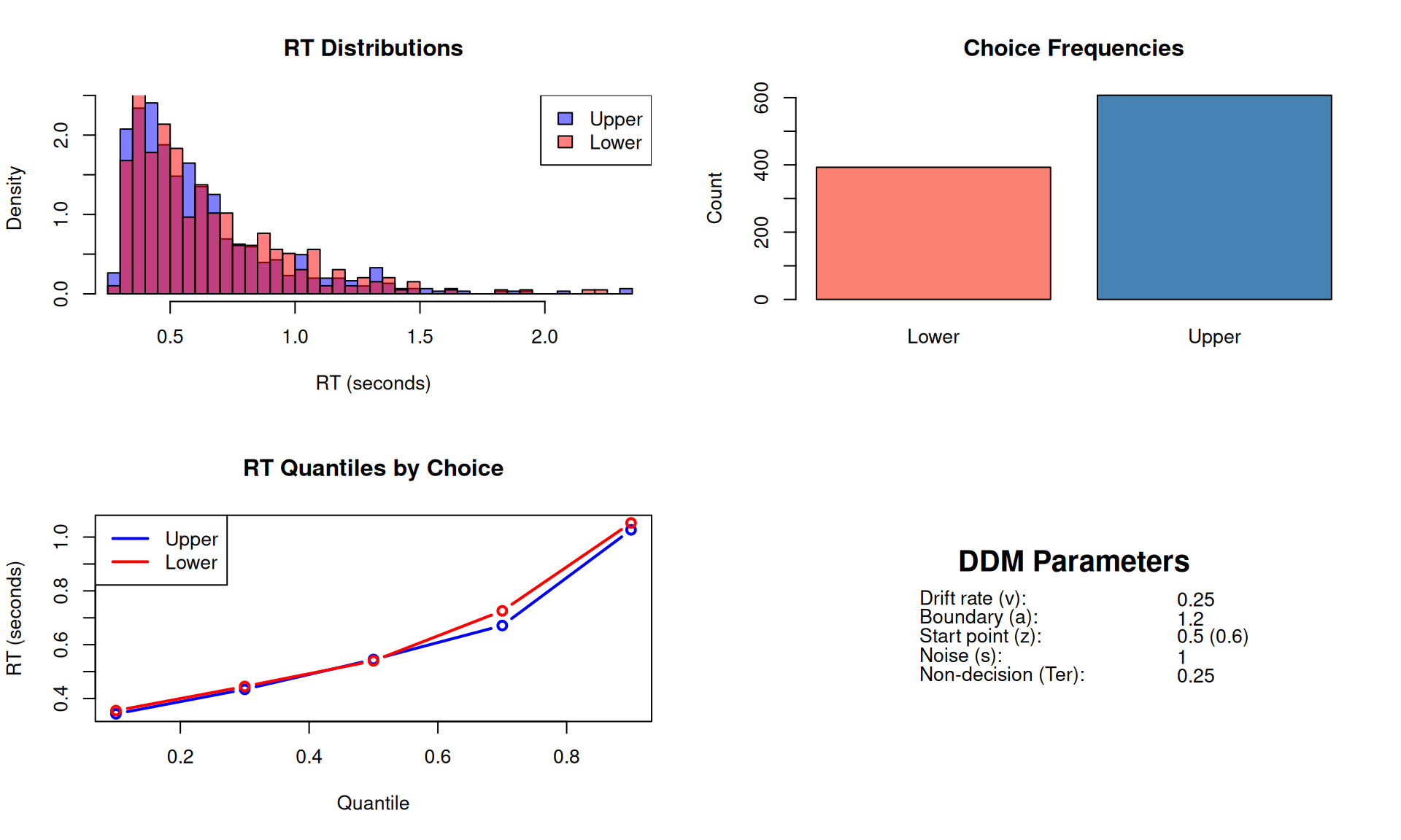

par(mfrow = c(1, 1))

1. Random walk → pure noise, no direction 2. Add drift → systematic tendency 3. Add boundaries → decisions emerge 4. Add non-decision time → realistic RTs 5. Complete DDM → accounts for accuracy AND RT

Drift Diffusion Model

Random Walk to Full Model

2025

STEP 1: Pure Random Walk - The Foundation

Mathematical Formulation

Direct Simulation Code

Multiple Paths to See Variability

STEP 2: Adding Drift - Systematic Tendency

Mathematical Formulation

Direct Simulation with Drift

Compare Different Drift Values

STEP 3: From Discrete to Continuous Time

Mathematical Formulation

Direct Simulation in Continuous Time

STEP 4: Adding Decision Boundaries

Mathematical Formulation

Direct Simulation with Boundaries

Key Observations

Simulate Multiple Trials

STEP 5: Adding Non-Decision Time

Mathematical Formulation

Simulation with Non-Decision Time

STEP 6: The Complete DDM

Mathematical Formulation

Complete DDM Simulation